Theta-cycle detection tutorial¶

Detect theta cycles from one LFP channel and inspect the saved CellExplorer-compatible events. The session path matches lfp_loader_tutorial.ipynb.

%matplotlib inline
%config InlineBackend.figure_format = 'retina'

import matplotlib.pyplot as plt
import numpy as np

import neuro_py as npy

npy.plotting.set_plotting_defaults()

1. Set the session path¶

Set basepath to the same session used in the LFP loader tutorial. It must contain the LFP recording, XML metadata, and channel annotations used to choose a theta channel.

basepath = r"U:\data\hpc_ctx_project\HP18\hp18_day85_20250713"

2. Load one theta channel¶

LFPLoader accesses a single channel without loading the full recording. The channel is selected from the CA1so annotation, matching the detector's default preference.

brain_regions = npy.io.load_brain_regions(basepath, out_format="DataFrame")
theta_channel = int(brain_regions.query("region == 'CA1so'").channels.iloc[0])
theta_lfp = npy.io.LFPLoader(basepath, channels=theta_channel, ext="lfp")
times = theta_lfp.abscissa_vals
signal = theta_lfp.data[0]
print(f"theta channel: {theta_channel}; sampling rate: {theta_lfp.fs} Hz")

theta channel: 175; sampling rate: 1250 Hz

3. Inspect the raw trace¶

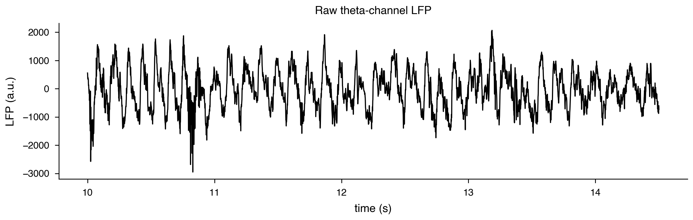
A short raw window verifies that the selected channel contains an oscillatory signal before running the full-session detector.

window_start = float(times[0] + 10.0)
window_stop = window_start + 4.5
window = (times >= window_start) & (times <= window_stop)

fig, ax = plt.subplots(
    figsize=npy.plotting.set_size(width="nature_double", ratio=0.25), dpi=200
)
ax.plot(times[window], signal[window], color="black", lw=0.7)
ax.set(xlabel="time (s)", ylabel="LFP (a.u.)", title="Raw theta-channel LFP")
plt.show()

png

4. Detect and reload theta cycles¶

get_theta_cycles detects cycles over the session and writes the standard .thetacycles.events.mat file. Reloading through npy.io gives the cycle boundaries and trough times used below.

npy.lfp.get_theta_cycles(basepath, ch=theta_channel)
theta_cycles = npy.io.load_theta_cycles(basepath)
theta_cycles.head()

	start	stop	duration	center	trough	theta_channel
0	0.2008	0.3464	0.1456	0.2736	0.2856	175
1	0.3464	0.5240	0.1776	0.4352	0.4536	175
2	0.5240	0.6920	0.1680	0.6080	0.6536	175
3	1.6560	1.8264	0.1704	1.7412	1.7400	175
4	1.8264	1.9336	0.1072	1.8800	1.8704	175

5. Overlay detected cycle boundaries and troughs¶

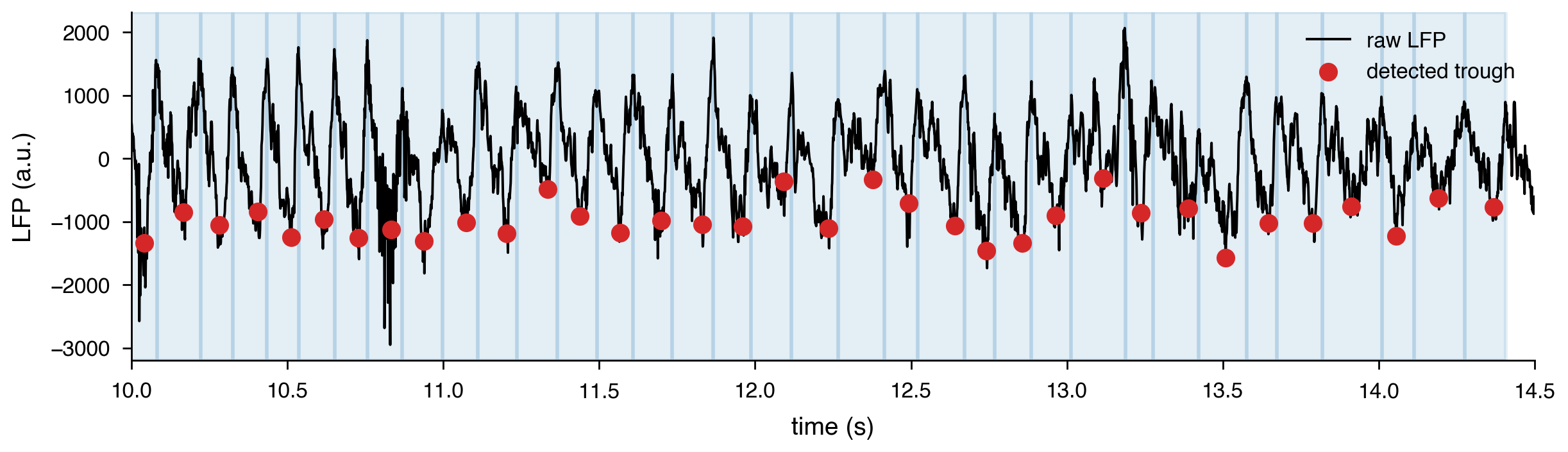
The boundary lines and trough markers should align with the visible theta rhythm in the raw trace. This is a direct visual check of the detector output.

cycles_in_window = theta_cycles.query("start <= @window_stop and stop >= @window_start")

fig, ax = plt.subplots(
    figsize=npy.plotting.set_size(width="nature_double", ratio=0.25), dpi=200
)
ax.plot(times[window], signal[window], color="black", lw=0.7, label="raw LFP")
for start, stop in cycles_in_window[["start", "stop"]].to_numpy():
    ax.axvspan(start, stop, color="tab:blue", alpha=0.12)
ax.scatter(
    cycles_in_window.trough,
    np.interp(cycles_in_window.trough, times, signal),
    color="tab:red",
    s=18,
    zorder=3,
    label="detected trough",
)
ax.set(xlim=(window_start, window_stop), xlabel="time (s)", ylabel="LFP (a.u.)")
ax.legend(frameon=False)
plt.show()

png