Posterior-weighted 2D regression¶

weighted_regression_2d fits a straight, constant-velocity trajectory to a posterior probability array with shape (x, y, time). It returns r2, x_traj, y_traj, slope_x, slope_y, mean_x, mean_y.

The fit minimizes posterior-weighted squared Euclidean residuals: \(\hat{\mathbf p}(t)=\bar{\mathbf p}+\mathbf b(t-\bar t)\). The variance-weighted multivariate coefficient of determination is

\[R^2=1-\frac{\mathrm{SSE}}{\mathrm{SST}} =\frac{\operatorname{Cov}_w(X,T)^2+\operatorname{Cov}_w(Y,T)^2} {\operatorname{Var}_w(T)[\operatorname{Var}_w(X)+\operatorname{Var}_w(Y)]}.\]

The first returned value is R², the fraction of total spatial variance explained by the fitted line, in [0,1]. It is unsigned. Slopes encode direction; the last two outputs are spatial means, not regression intercepts. The fitted trajectory is distinct from the posterior center of mass.

Use the same physical units for x and y for rotation invariance. Normalize each time slice to one for equal temporal weighting. Synthetic examples below need no external data; the final real-data workflow is optional.

Reading guide¶

The simulations vary one aspect at a time:

Direction: establish that the fit is independent of trajectory angle.
Uncertainty: keep ordered movement and increase posterior spread or noise.
Negative controls: remove ordered movement and compare with signal plus noise.
Model limitations: introduce curvature and repeated jumps.

Every example includes the same 500-shuffle test. Read R² as fit magnitude and the p-value as evidence relative to the specified null. Helper definitions come first; optional edge cases, timing, and real data follow the main sequence.

import matplotlib
import matplotlib.cm as mpl_cm
import matplotlib.colors as colors
import matplotlib.pyplot as plt
import nelpy as nel
import numpy as np
import pandas as pd

import neuro_py as npy
from neuro_py.ensemble.replay import weighted_regression_2d

R² magnitude and shuffle significance¶

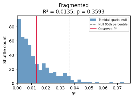
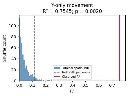
R² describes explained spatial variance; its size alone does not establish whether an event is unusual under a null model. A diffuse linear posterior can explain little total variance yet have more temporal structure than its shuffles. Each simulation below includes an observed-versus-null histogram.

The self-contained helper reproduces hpc_ctx.replay.replay_2d's axis_wise_toroidal method: independently translate each spatial posterior by random x/y offsets, wrapping at the arena boundaries. This preserves per-bin probability values, total mass, and shape on the torus while disrupting the spatial alignment between time bins.

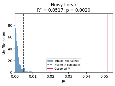
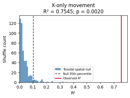
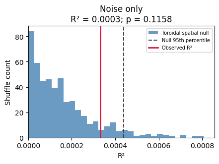
We use 500 shuffles and a fixed seed. The upper-tail Monte Carlo p-value is (1 + number of shuffled R² >= observed R²) / (1 + n_shuffles), including ties. Its minimum is 1/501 (approximately 0.002). The dashed line marks the null 95th percentile; p-values provide the decision rule at the chosen alpha.

These are illustrative, unadjusted per-simulation p-values under this specific null, not proof of biological replay. Toroidal shifts assume a wraparound geometry, and independent bin shifts remove temporal dependence. Real arena boundaries and overlapping decode windows still require separate null calibration. The simulated posteriors here do not use overlapping spike count windows.

N_SHUFFLES = 500
SHUFFLE_SEED = 42


def toroidal_spatial_shuffle(posterior, x_shifts, y_shifts):
    """Translate each spatial posterior independently on a 2D torus."""
    shuffled = np.empty_like(posterior)
    for k in range(posterior.shape[2]):
        shuffled[:, :, k] = np.roll(
            posterior[:, :, k], shift=(x_shifts[k], y_shifts[k]), axis=(0, 1)
        )
    return shuffled


def r2_shuffle_test(posterior, n_shuffles=N_SHUFFLES, seed=SHUFFLE_SEED):
    """Return observed R², the spatial null, and its upper-tail Monte Carlo p."""
    if not isinstance(n_shuffles, (int, np.integer)) or n_shuffles < 1:
        raise ValueError("n_shuffles must be a positive integer")
    observed = weighted_regression_2d(posterior)[0]
    rng = np.random.default_rng(seed)
    nx, ny, nt = posterior.shape
    null = np.empty(n_shuffles)
    for b in range(n_shuffles):
        x_shifts = rng.integers(0, nx, size=nt)
        y_shifts = rng.integers(0, ny, size=nt)
        null[b] = weighted_regression_2d(
            toroidal_spatial_shuffle(posterior, x_shifts, y_shifts)
        )[0]
    if not np.isfinite(observed) or not np.all(np.isfinite(null)):
        raise ValueError("Observed and shuffled R² must be finite for this test")
    p_value = (1 + np.count_nonzero(null >= observed)) / (n_shuffles + 1)
    return observed, null, p_value


def plot_r2_nulls(simulations, n_shuffles=N_SHUFFLES, seed=SHUFFLE_SEED):
    """Plot each simulation against its null and return a numeric summary."""
    ncols = min(3, len(simulations))
    nrows = (len(simulations) + ncols - 1) // ncols
    fig, axes = plt.subplots(
        nrows,
        ncols,
        figsize=(4.3 * ncols, 3.2 * nrows),
        squeeze=False,
        constrained_layout=True,
    )
    streams = np.random.SeedSequence(seed).spawn(len(simulations))
    rows = []
    for ax, (name, posterior), stream in zip(axes.flat, simulations.items(), streams):
        observed, null, p_value = r2_shuffle_test(posterior, n_shuffles, stream)
        q95 = np.quantile(null, 0.95)
        ax.hist(
            null, bins=30, color="steelblue", alpha=0.8, label="Toroidal spatial null"
        )
        ax.axvline(q95, color="0.25", ls="--", lw=1.4, label="Null 95th percentile")
        ax.axvline(observed, color="crimson", lw=2, label="Observed R²")
        upper = max(observed, null.max())
        ax.set(
            title=f"{name}\nR² = {observed:.4f}; p = {p_value:.4f}",
            xlabel="R²",
            ylabel="Shuffle count",
            xlim=(0, 1.06 * upper if upper > 0 else 0.01),
        )
        ax.legend(fontsize=7)
        rows.append(
            {
                "simulation": name,
                "observed_r2": observed,
                "null_95th_percentile": q95,
                "p_value": p_value,
                "n_shuffles": n_shuffles,
            }
        )
    for ax in axes.flat[len(simulations) :]:
        ax.set_visible(False)
    plt.show()
    return pd.DataFrame(rows).set_index("simulation")

Simulation setup¶

All helpers normalize each spatial slice to total probability one, so every decode bin receives equal weight. Noise seeds are fixed for reproducibility. The finite-uncertainty angle and spread comparisons match speeds and avoid arena edges.

def simulate_degenerate_x(t_dim=20, x_fixed=5, noise=0.01):
    """All weight on a single x row — trajectory moves only in Y."""
    rng = np.random.default_rng(42)
    x_dim, y_dim = 10, 10
    weights = np.zeros((x_dim, y_dim, t_dim), dtype=np.float64)
    for k in range(t_dim):
        cy = k / (t_dim - 1) * (y_dim - 1)
        for j in range(y_dim):
            weights[x_fixed, j, k] = np.exp(-((j - cy) ** 2) / 4.0)
    weights[x_fixed] += rng.uniform(0, noise, (y_dim, t_dim))
    return weights / weights.sum(axis=(0, 1), keepdims=True)


def simulate_degenerate_y(t_dim=20, y_fixed=5, noise=0.01):
    """All weight on a single y column — trajectory moves only in X."""
    rng = np.random.default_rng(42)
    x_dim, y_dim = 10, 10
    weights = np.zeros((x_dim, y_dim, t_dim), dtype=np.float64)
    for k in range(t_dim):
        cx = k / (t_dim - 1) * (x_dim - 1)
        for i in range(x_dim):
            weights[i, y_fixed, k] = np.exp(-((i - cx) ** 2) / 4.0)
    weights[:, y_fixed, :] += rng.uniform(0, noise, (x_dim, t_dim))
    return weights / weights.sum(axis=(0, 1), keepdims=True)


def simulate_no_movement(t_dim=20, noise=0.01):
    """Weight fixed at a single spatial location — no temporal drift."""
    rng = np.random.default_rng(42)
    x_dim, y_dim = 10, 10
    weights = np.zeros((x_dim, y_dim, t_dim), dtype=np.float64)
    weights[5, 5, :] = 1.0
    weights += rng.uniform(0, noise, (x_dim, y_dim, t_dim))
    return weights / weights.sum(axis=(0, 1), keepdims=True)


def simulate_both_axes(t_dim=20, noise=0.01):
    """Weight drifts diagonally — both X and Y move over time."""
    rng = np.random.default_rng(42)
    x_dim, y_dim = 10, 10
    weights = np.zeros((x_dim, y_dim, t_dim), dtype=np.float64)
    for k in range(t_dim):
        cx = k / (t_dim - 1) * (x_dim - 1)
        cy = k / (t_dim - 1) * (y_dim - 1)
        for i in range(x_dim):
            for j in range(y_dim):
                weights[i, j, k] = np.exp(-((i - cx) ** 2 + (j - cy) ** 2) / 4.0)
    weights += rng.uniform(0, noise, weights.shape)
    return weights / weights.sum(axis=(0, 1), keepdims=True)


def simulate_anti_diagonal(t_dim=20, noise=0.01):
    """Weight drifts along an anti-diagonal — both X and Y move over time."""
    rng = np.random.default_rng(42)
    x_dim, y_dim = 10, 10
    weights = np.zeros((x_dim, y_dim, t_dim), dtype=np.float64)
    for k in range(t_dim):
        cx = k / (t_dim - 1) * (x_dim - 1)
        cy = (y_dim - 1) - k / (t_dim - 1) * (y_dim - 1)
        for i in range(x_dim):
            for j in range(y_dim):
                weights[i, j, k] = np.exp(-((i - cx) ** 2 + (j - cy) ** 2) / 4.0)
    weights += rng.uniform(0, noise, weights.shape)
    return weights / weights.sum(axis=(0, 1), keepdims=True)


def simulate_curved(t_dim=20, noise=0.05):
    """Trajectory follows a curved arc (sine wave in Y)."""
    rng = np.random.default_rng(42)
    x_dim, y_dim = 10, 10
    weights = np.zeros((x_dim, y_dim, t_dim), dtype=np.float64)
    for k in range(t_dim):
        cx = k / (t_dim - 1) * (x_dim - 1)
        cy = 4.5 + 4.0 * np.sin(np.pi * k / (t_dim - 1))  # arc from 4.5 -> peak -> 4.5
        for i in range(x_dim):
            for j in range(y_dim):
                weights[i, j, k] = np.exp(-((i - cx) ** 2 + (j - cy) ** 2) / 2.0)
    weights += rng.uniform(0, noise, weights.shape)
    return weights / weights.sum(axis=(0, 1), keepdims=True)


def simulate_noisy_linear(t_dim=20, noise=0.15):
    """Linear trajectory with substantial noise — realistic decode uncertainty."""
    rng = np.random.default_rng(42)
    x_dim, y_dim = 10, 10
    weights = np.zeros((x_dim, y_dim, t_dim), dtype=np.float64)
    for k in range(t_dim):
        cx = k / (t_dim - 1) * (x_dim - 1)
        cy = k / (t_dim - 1) * (y_dim - 1)
        for i in range(x_dim):
            for j in range(y_dim):
                weights[i, j, k] = np.exp(-((i - cx) ** 2 + (j - cy) ** 2) / 4.0)
    weights += rng.uniform(0, noise, weights.shape)
    return weights / weights.sum(axis=(0, 1), keepdims=True)


def simulate_reverse(t_dim=20, noise=0.01):
    """Trajectory moves from high to low — tests signed slopes with unsigned R²."""
    rng = np.random.default_rng(42)
    x_dim, y_dim = 10, 10
    weights = np.zeros((x_dim, y_dim, t_dim), dtype=np.float64)
    for k in range(t_dim):
        cx = (x_dim - 1) - k / (t_dim - 1) * (x_dim - 1)  # 9 -> 0
        cy = (y_dim - 1) - k / (t_dim - 1) * (y_dim - 1)  # 9 -> 0
        for i in range(x_dim):
            for j in range(y_dim):
                weights[i, j, k] = np.exp(-((i - cx) ** 2 + (j - cy) ** 2) / 4.0)
    weights += rng.uniform(0, noise, weights.shape)
    return weights / weights.sum(axis=(0, 1), keepdims=True)


def simulate_fragmented(t_dim=20, noise=0.05):
    """Weight jumps between two spatial clusters — fragmented/ambiguous replay."""
    rng = np.random.default_rng(42)
    x_dim, y_dim = 10, 10
    weights = np.zeros((x_dim, y_dim, t_dim), dtype=np.float64)
    for k in range(t_dim):
        # Alternate between two clusters
        if k % 4 < 2:
            cx, cy = 2.0, 2.0
        else:
            cx, cy = 7.0, 7.0
        for i in range(x_dim):
            for j in range(y_dim):
                weights[i, j, k] = np.exp(-((i - cx) ** 2 + (j - cy) ** 2) / 2.0)
    weights += rng.uniform(0, noise, weights.shape)
    return weights / weights.sum(axis=(0, 1), keepdims=True)


def simulate_noise_only(t_dim=20, seed=42):
    """Independent background noise with no moving spatial signal."""
    rng = np.random.default_rng(seed)
    weights = rng.uniform(0, 0.50, (10, 10, t_dim))
    return weights / weights.sum(axis=(0, 1), keepdims=True)


def helper_plot(weights):
    fig, ax = plt.subplots(1, weights.shape[2], figsize=(20, 2))
    vmax = np.percentile(weights, 99.9)
    for i in range(weights.shape[2]):
        ax[i].imshow(
            weights[..., i].T, origin="lower", aspect="equal", vmin=0, vmax=vmax
        )
        ax[i].set_title(f"t={i}")
    plt.show()

def equal_speed_posterior(dx, dy, spread=1):
    posterior = np.zeros((65, 65, 9))
    offsets = np.arange(-2, 3)
    mass = np.exp(-(offsets**2) / (2 * spread**2))
    mass /= mass.sum()
    for k in range(9):
        posterior[np.ix_(10 + dx * k + offsets, 10 + dy * k + offsets, [k])] = (
            mass[:, None] * mass[None, :]
        )[..., None]
    return posterior

1. Direction: establish the baseline¶

1.1 Perfectly localized straight motion¶

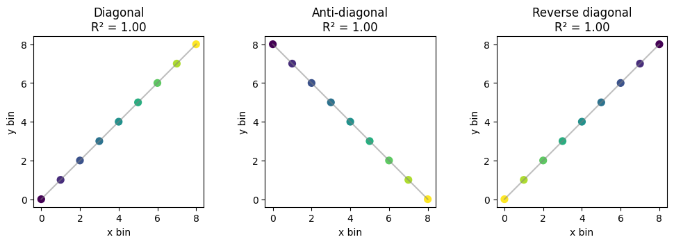
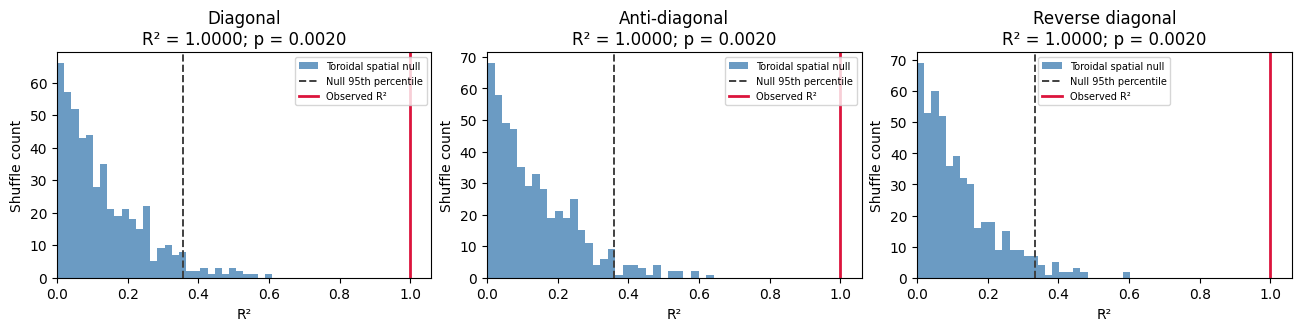
Start with no spatial uncertainty. Diagonal, anti-diagonal, and reversed paths all have R² = 1; direction is represented by the signed slopes.

n = 9
diagonal = np.zeros((n, n, n))
diagonal[np.arange(n), np.arange(n), np.arange(n)] = 1
examples = {
    "Diagonal": diagonal,
    "Anti-diagonal": diagonal[:, ::-1, :],
    "Reverse diagonal": diagonal[..., ::-1],
}
rows = []
fig, axes = plt.subplots(1, 3, figsize=(10, 3.4), constrained_layout=True)
for ax, (name, posterior) in zip(axes, examples.items()):
    r2, x_fit, y_fit, vx, vy, mx, my = weighted_regression_2d(posterior)
    rows.append({"trajectory": name, "R²": r2, "slope_x": vx, "slope_y": vy})
    np.testing.assert_allclose(r2, 1, atol=1e-12)
    ax.scatter(x_fit, y_fit, c=np.arange(n), cmap="viridis", s=50)
    ax.plot(x_fit, y_fit, color="0.5", alpha=0.5)
    ax.set(title=f"{name}\nR² = {r2:.2f}", xlabel="x bin", ylabel="y bin")
    ax.set_aspect("equal")
display(pd.DataFrame(rows).set_index("trajectory"))
plt.show()

display(plot_r2_nulls(examples))

	R²	slope_x	slope_y
trajectory
Diagonal	1.0	1.0	1.0
Anti-diagonal	1.0	1.0	-1.0
Reverse diagonal	1.0	-1.0	-1.0

png

	observed_r2	null_95th_percentile	p_value	n_shuffles
simulation
Diagonal	1.0	0.358077	0.001996	500
Anti-diagonal	1.0	0.360742	0.001996	500
Reverse diagonal	1.0	0.332554	0.001996	500

1.2 Change direction while matching speed and uncertainty¶

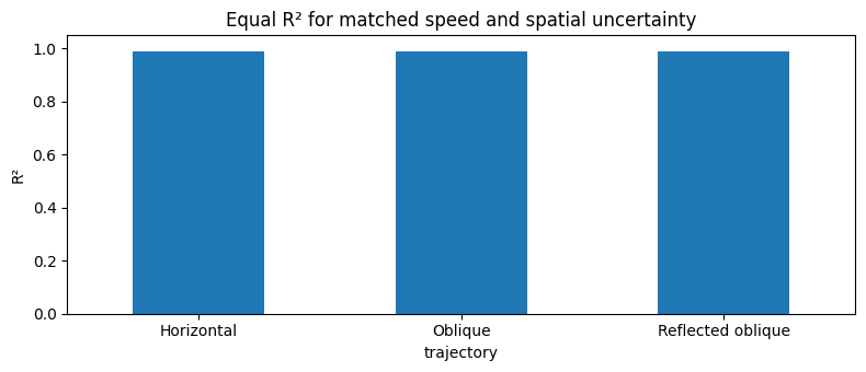
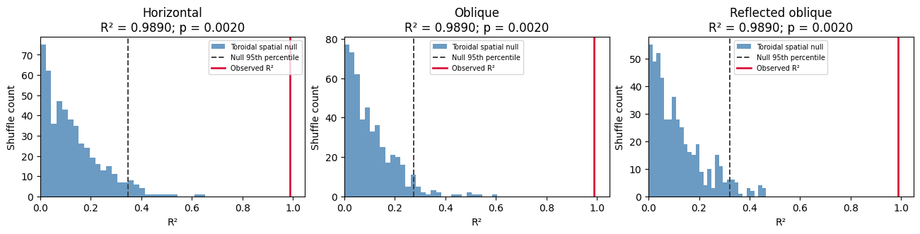
Horizontal velocity (5,0) and oblique velocity (3,4) have equal magnitude. Both use the same symmetric isotropic uncertainty. Reflection changes direction without changing fit magnitude. Integer coordinates avoid spatial interpolation artifacts, and the paths stay away from arena boundaries.

horizontal = equal_speed_posterior(5, 0)
oblique = equal_speed_posterior(3, 4)
matched = {
    "Horizontal": horizontal,
    "Oblique": oblique,
    "Reflected oblique": oblique[:, ::-1],
}
rotation_table = pd.DataFrame(
    [
        {"trajectory": name, "R²": weighted_regression_2d(p)[0]}
        for name, p in matched.items()
    ]
).set_index("trajectory")
np.testing.assert_allclose(
    rotation_table["R²"], rotation_table["R²"].iloc[0], atol=1e-12
)
display(rotation_table)
rotation_table.plot.bar(
    rot=0, ylim=(0, 1.05), ylabel="R²", figsize=(8, 3.5), legend=False
)
plt.title("Equal R² for matched speed and spatial uncertainty")
plt.tight_layout()
plt.show()


display(plot_r2_nulls(matched))

	R²
trajectory
Horizontal	0.98903
Oblique	0.98903
Reflected oblique	0.98903

png

	observed_r2	null_95th_percentile	p_value	n_shuffles
simulation
Horizontal	0.98903	0.348691	0.001996	500
Oblique	0.98903	0.272963	0.001996	500
Reflected oblique	0.98903	0.322592	0.001996	500

2. Uncertainty: preserve the ordered trajectory¶

2.1 Broaden the spatial posterior¶

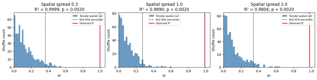
Hold the oblique trajectory fixed and vary only the spatial spread parameter. R² decreases because spatial uncertainty contributes unexplained variance. The finite spatial kernel is identical across examples except for its spread.

# Posterior spread is retained in the residual, unlike scoring only its mean.
uncertainty = pd.DataFrame(
    [
        {
            "spread": spread,
            "R²": weighted_regression_2d(equal_speed_posterior(3, 4, spread))[0],
        }
        for spread in (0.3, 1.0, 2.0)
    ]
)
assert np.all(np.diff(uncertainty["R²"]) < 0)
display(uncertainty)


display(
    plot_r2_nulls(
        {
            f"Spatial spread {spread}": equal_speed_posterior(3, 4, spread)
            for spread in (0.3, 1.0, 2.0)
        }
    )
)

	spread	R²
0	0.3	0.999908
1	1.0	0.989030
2	2.0	0.980429

png

	observed_r2	null_95th_percentile	p_value	n_shuffles
simulation
Spatial spread 0.3	0.999908	0.364154	0.001996	500
Spatial spread 1.0	0.989030	0.272963	0.001996	500
Spatial spread 2.0	0.980429	0.341145	0.001996	500

2.2 A linear trajectory with little background noise¶

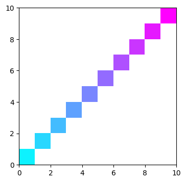
This is the baseline for the next example: a moving Gaussian spatial signal plus a small background-noise component. The trajectory remains ordered.

weights = simulate_both_axes()
r2, x_traj, y_traj, slope_x, slope_y, mean_x, mean_y = weighted_regression_2d(weights)

print(f"R²   : {r2:.4f}")
print(f"slope_x             : {slope_x:.4f}")
print(f"slope_y             : {slope_y:.4f}")

helper_plot(weights)
npy.plotting.plot_2d_replay(weights)
plt.show()

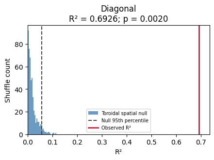
null_summary = plot_r2_nulls({"Diagonal": weights})
display(null_summary)

R²   : 0.6926
slope_x             : 0.3924
slope_y             : 0.3921

png

	observed_r2	null_95th_percentile	p_value	n_shuffles
simulation
Diagonal	0.692552	0.057315	0.001996	500

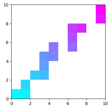
2.3 Increase background noise while retaining the signal¶

Keep the moving Gaussian signal and increase the background noise. The posterior becomes diffuse, reducing R². The histogram tests whether that remaining linear structure is unusual relative to the toroidal null. Low R² does not automatically imply nonsignificance, but it still means that much of the spatial variance is unexplained.

weights = simulate_noisy_linear(noise=0.50)
r2, x_traj, y_traj, slope_x, slope_y, mean_x, mean_y = weighted_regression_2d(weights)

print(f"R²   : {r2:.4f}  (lower than clean diagonal due to noise)")
print(f"slope_x             : {slope_x:.4f}")
print(f"slope_y             : {slope_y:.4f}")

helper_plot(weights)
npy.plotting.plot_2d_replay(weights)
plt.show()

signal_noise_summary = plot_r2_nulls({"Noisy linear": weights})
display(signal_noise_summary)

R²   : 0.0517  (lower than clean diagonal due to noise)
slope_x             : 0.1127
slope_y             : 0.1076

png

	observed_r2	null_95th_percentile	p_value	n_shuffles
simulation
Noisy linear	0.051652	0.004804	0.001996	500

3. Negative controls: remove ordered movement¶

3.1 Background noise alone¶

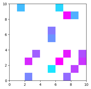
Remove the moving Gaussian signal, retaining the same fixed-seed noise component used in section 2.3 before normalization. Each time slice is an independent random spatial distribution. This is a matched signal-present versus signal-absent comparison, not just a larger noise amplitude.

With the supplied seeds, this control does not pass the 0.05 shuffle threshold. The table compares its measured p-value with the noisy linear example. Noise realizations can occasionally pass a test by chance; the seed is fixed, and the code neither searches seeds nor forces a nonsignificant result.

weights = simulate_noise_only()
r2, x_traj, y_traj, slope_x, slope_y, mean_x, mean_y = weighted_regression_2d(weights)
print(f"R²: {r2:.4f}")
helper_plot(weights)
npy.plotting.plot_2d_replay(weights)
plt.show()
noise_only_summary = plot_r2_nulls({"Noise only": weights})
display(noise_only_summary)

noise_comparison = pd.concat([signal_noise_summary, noise_only_summary])
noise_comparison["p < 0.05"] = noise_comparison["p_value"] < 0.05
display(noise_comparison)

R²: 0.0003

png

	observed_r2	null_95th_percentile	p_value	n_shuffles
simulation
Noise only	0.000331	0.00044	0.115768	500

	observed_r2	null_95th_percentile	p_value	n_shuffles	p < 0.05
simulation
Noisy linear	0.051652	0.004804	0.001996	500	True
Noise only	0.000331	0.000440	0.115768	500	False

3.2 Spatial concentration without movement¶

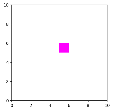
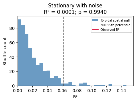
A stationary spatial peak with small background noise tests a different negative control: localization alone is not evidence of a linear sequence.

weights = simulate_no_movement()
r2, x_traj, y_traj, slope_x, slope_y, mean_x, mean_y = weighted_regression_2d(weights)

print(f"R²   : {r2:.4f}  (expect ~0, no signal)")
print(f"slope_x             : {slope_x:.3e}")
print(f"slope_y             : {slope_y:.3e}")

helper_plot(weights)
npy.plotting.plot_2d_replay(weights)
plt.show()

null_summary = plot_r2_nulls({"Stationary with noise": weights})
display(null_summary)

R²   : 0.0001  (expect ~0, no signal)
slope_x             : 3.815e-03
slope_y             : 1.324e-03

png

	observed_r2	null_95th_percentile	p_value	n_shuffles
simulation
Stationary with noise	0.000096	0.061809	0.994012	500

4. Model limitations: depart from a straight trajectory¶

4.1 Smooth curvature¶

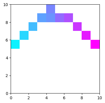
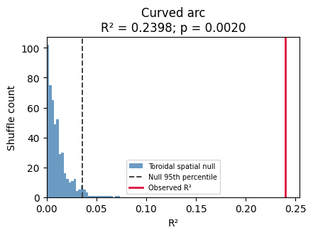
A smooth arc contains ordered movement, but a constant-velocity line cannot explain all of it. Inspect both R² and the shuffle result: significance does not imply that the linear model describes the complete path.

weights = simulate_curved()
r2, x_traj, y_traj, slope_x, slope_y, mean_x, mean_y = weighted_regression_2d(weights)

print(f"R²   : {r2:.4f}  (attenuated vs diagonal — nonlinear Y)")
print(f"slope_x             : {slope_x:.4f}  (X is still linear)")
print(f"slope_y             : {slope_y:.4f}  (near 0 — arc cancels out)")

helper_plot(weights)
npy.plotting.plot_2d_replay(weights)
plt.show()

null_summary = plot_r2_nulls({"Curved arc": weights})
display(null_summary)

R²   : 0.2398  (attenuated vs diagonal — nonlinear Y)
slope_x             : 0.3072  (X is still linear)
slope_y             : 0.0012  (near 0 — arc cancels out)

png

	observed_r2	null_95th_percentile	p_value	n_shuffles
simulation
Curved arc	0.239764	0.035767	0.001996	500

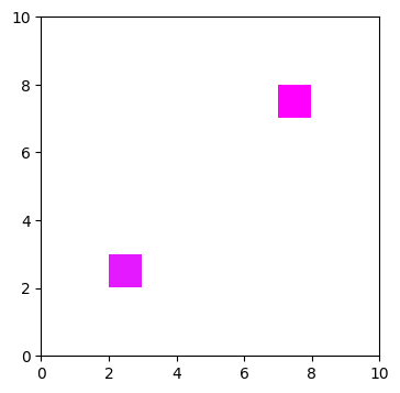
4.2 Repeated jumps between locations¶

Repeated back-and-forth jumps produce little net linear progression in this example, despite concentrated spatial probability. Other discontinuous paths can have substantial R². Neither R² nor a shuffle p-value alone establishes trajectory continuity.

weights = simulate_fragmented()
r2, x_traj, y_traj, slope_x, slope_y, mean_x, mean_y = weighted_regression_2d(weights)

print(f"R²   : {r2:.4f}  (linear fit across two clusters)")
print(f"slope_x             : {slope_x:.4f}")
print(f"slope_y             : {slope_y:.4f}")

helper_plot(weights)
npy.plotting.plot_2d_replay(weights)
plt.show()

null_summary = plot_r2_nulls({"Fragmented": weights})
display(null_summary)

R²   : 0.0135  (linear fit across two clusters)
slope_x             : 0.0561
slope_y             : 0.0539

png

	observed_r2	null_95th_percentile	p_value	n_shuffles
simulation
Fragmented	0.013464	0.036332	0.359281	500

Interpretation¶

Scenario	R²	Interpretation
Perfect localized line, any direction	1	All spatial variance explained
Stationary diffuse posterior	0	No linear temporal movement
Independent background noise	Usually small	No designed temporal sequence; assess the empirical p-value
Stationary point mass	NaN	Total spatial variance is zero
Broader posterior, same moving mean	Lower	Uncertainty contributes residual variance
Time reversal	Unchanged	Slopes change sign
Curved or reversing path	Often lower	A single constant-velocity line is incomplete
Fragmented path	Can be substantial	R² alone does not establish continuity

NaNs contribute zero weight. Keep original timestamps when removing time bins; do not compress gaps. Negative and infinite weights are invalid. R² is undefined for zero total weight or zero temporal or spatial variance. Compare event R² against an upper-tail shuffle distribution to assess significance. Selection of a suitable null is separate from regression fit.

Optional edge cases: movement confined to one axis¶

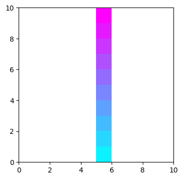
These checks place all probability on a single x row or y column. One spatial coordinate has zero variance; the moving coordinate still supports a well-defined regression. They complement the main direction comparisons.

Fixed x, movement in y¶

weights = simulate_degenerate_x()
r2, x_traj, y_traj, slope_x, slope_y, mean_x, mean_y = weighted_regression_2d(weights)

print(f"R²   : {r2:.4f}")
print(f"slope_x             : {slope_x:.3e}  (expect ~0)")
print(f"slope_y             : {slope_y:.4f}")

helper_plot(weights)
npy.plotting.plot_2d_replay(weights)
plt.show()

null_summary = plot_r2_nulls({"Y-only movement": weights})
display(null_summary)

R²   : 0.7545
slope_x             : -4.474e-17  (expect ~0)
slope_y             : 0.4099

png

	observed_r2	null_95th_percentile	p_value	n_shuffles
simulation
Y-only movement	0.754473	0.114447	0.001996	500

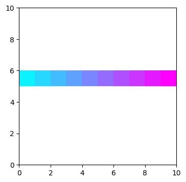
Fixed y, movement in x¶

weights = simulate_degenerate_y()
r2, x_traj, y_traj, slope_x, slope_y, mean_x, mean_y = weighted_regression_2d(weights)

print(f"R²   : {r2:.4f}")
print(f"slope_x             : {slope_x:.4f}")
print(f"slope_y             : {slope_y:.3e}  (expect ~0)")
helper_plot(weights)

npy.plotting.plot_2d_replay(weights)
plt.show()

null_summary = plot_r2_nulls({"X-only movement": weights})
display(null_summary)

R²   : 0.7545
slope_x             : 0.4099
slope_y             : -4.474e-17  (expect ~0)

png

	observed_r2	null_95th_percentile	p_value	n_shuffles
simulation
X-only movement	0.754473	0.10342	0.001996	500

Warmed-up performance¶

The Numba kernel scans the posterior once, uses float64 accumulators, and allocates only small marginal arrays. It releases the GIL and avoids per-event parallel dispatch. Timing excludes first-call JIT compilation and includes the public wrapper and trajectory outputs. Measurements below are machine-specific, not an end-to-end replay runtime guarantee.

import timeit

benchmark_rows = []
for dtype in (np.float32, np.float64):
    for layout in ("C", "F"):
        p = np.random.default_rng(42).random((50, 50, 20)).astype(dtype)
        p /= p.sum(axis=(0, 1), keepdims=True)
        p = np.array(p, order=layout)
        weighted_regression_2d(p)  # compile/warm up this signature
        seconds = (
            min(timeit.repeat(lambda: weighted_regression_2d(p), number=1000, repeat=3))
            / 1000
        )
        benchmark_rows.append(
            {
                "dtype": np.dtype(dtype).name,
                "layout": layout,
                "µs/event": seconds * 1e6,
                "events/s": 1 / seconds,
                "seconds/10,000 events": seconds * 10000,
            }
        )
display(pd.DataFrame(benchmark_rows))

	dtype	layout	µs/event	events/s	seconds/10,000 events
0	float32	C	154.7166	6463.430555	1.547166
1	float32	F	120.9882	8265.268844	1.209882
2	float64	C	132.6365	7539.402804	1.326365
3	float64	F	118.2131	8459.299349	1.182131

Optional real data¶

Enable RUN_REAL_DATA and edit basepath for an available session. The synthetic examples above are self-contained.

RUN_REAL_DATA = True

if RUN_REAL_DATA:
    # SET UP PARAMETERS FOR REAL DATA
    MIN_RIP_DUR = 0.04  # minimum duration of ripple events to include in analysis (exclude short events that may reflect noise/artifacts)
    MAX_RIP_DUR = 0.3  # maximum duration of ripple events to include in analysis (exclude long events that may reflect different phenomena)
    N_ACTIVE_CELLS = 10  # minimum number of active cells in a ripple event to be included in analysis
    POST_SLEEP_IDX = 3  # which post task is the example event in?
    TASK_EPOCH = 2  # which post task is the example event in?
    SPEED_THRES = 10  # running threshold to determine tuning curves
    S_BINSIZE = 2  # spatial bins in tuning curve
    TUNING_CURVE_SIGMA = 3
    SLIDE_BY = 0.005
    BIN_SIZE = 0.02

    basepath = r"R:\data\latentseq\RM10\rm10_day6_20250810"
    st, cm = npy.io.load_spikes(
        basepath, brainRegion="CA1", putativeCellType="Pyr|Int", remove_unstable=True
    )

    # load position and compute speed
    position = npy.io.load_animal_behavior(basepath)
    pos = nel.AnalogSignalArray(
        [position.x.values, position.y.values], timestamps=position.timestamps.values
    )
    speed = nel.utils.ddt_asa(pos, smooth=True, sigma=0.250, norm=True)

    # load epochs and ripple events
    epoch_df = npy.io.load_epoch(basepath)
    beh_epochs = nel.EpochArray(epoch_df[["startTime", "stopTime"]].values)
    ripples = npy.io.load_ripples_events(basepath, return_epoch_array=True)

    # ripples are at least X seconds long
    ripples = nel.EpochArray(
        ripples.data[
            (ripples.lengths >= MIN_RIP_DUR) & (ripples.lengths <= MAX_RIP_DUR)
        ],
    )
    # ripples have at least X active cells
    bst = npy.process.count_in_interval(st.data, ripples.starts, ripples.stops)
    ripples = nel.EpochArray(
        ripples.data[(bst > 0).sum(axis=0) > N_ACTIVE_CELLS],
    )

    st, display(epoch_df)

	name	startTime	stopTime	environment	manipulation	behavioralParadigm	stimuli	notes	basepath
0	rm10_probe_250810_092719	0.0000	452.65915	cheeseboard	NaN	NaN	NaN	NaN	R:\data\latentseq\RM10\rm10_day6_20250810
1	rm10_presleep_250810_094149	452.6592	6206.85435	sleep	NaN	NaN	NaN	NaN	R:\data\latentseq\RM10\rm10_day6_20250810
2	rm10_cheeseboard1_250810_112435	6206.8544	8223.35355	cheeseboard	NaN	NaN	NaN	NaN	R:\data\latentseq\RM10\rm10_day6_20250810
3	rm10_postsleep1_250810_120316	8223.3536	13941.93075	sleep	NaN	NaN	NaN	NaN	R:\data\latentseq\RM10\rm10_day6_20250810
4	rm10_cheeseboard2_250810_134434	13941.9308	16500.15795	cheeseboard	NaN	NaN	NaN	NaN	R:\data\latentseq\RM10\rm10_day6_20250810
5	rm10_postsleep2_250810_143203	16500.1580	22562.22515	sleep	NaN	NaN	NaN	NaN	R:\data\latentseq\RM10\rm10_day6_20250810

compute spatial tuning curves¶

if RUN_REAL_DATA:
    spatial_maps = npy.tuning.SpatialMap(
        pos[beh_epochs[TASK_EPOCH]],
        st[beh_epochs[TASK_EPOCH]],
        s_binsize=S_BINSIZE,
        speed=speed,
        speed_thres=SPEED_THRES,
        tuning_curve_sigma=TUNING_CURVE_SIGMA,
    )

decode and score replays¶

Note: This real-data section does not perform shuffling; this is just to demonstrate the function on real data. In practice you would want to compare these scores to a shuffle distribution to determine significance.

if RUN_REAL_DATA:

    def jump_distance(posterior):
        # if single time bin return nan
        if posterior.shape[2] == 1:
            return np.nan, np.nan

        com = npy.ensemble.position_estimator(
            posterior.T,
            np.arange(posterior.shape[1]),
            np.arange(posterior.shape[0]),
            method="com",
        )
        # get spatial diff over time bins
        x_diff = np.diff(com[:, 0])
        y_diff = np.diff(com[:, 1])
        delta = np.sqrt(x_diff**2 + y_diff**2)
        max_jump = np.max(np.abs(delta))
        jump = np.sum(np.abs(delta)) / len(delta)

        return max_jump, jump

    # replays from task
    current_replays = ripples[beh_epochs[TASK_EPOCH]]

    bin_edges = npy.process.intervals.get_overlapping_intervals(
        current_replays.start - BIN_SIZE,
        current_replays.stop + BIN_SIZE,
        BIN_SIZE,
        SLIDE_BY,
    )
    bin_centers = np.mean(bin_edges, axis=1)

    bst = npy.process.count_in_interval(
        st.data,
        bin_edges[:, 0],
        bin_edges[:, 1],
    )

    # find which bin belongs to which ripple
    within_ripple_idx, within_ripple_ind = npy.process.in_intervals(
        bin_centers, current_replays.data, return_interval=True
    )
    ripple_index = within_ripple_ind[within_ripple_idx]
    unique_ripples = np.unique(ripple_index).astype(int)
    # remake current_replays in case of non unique ripples
    current_replays = nel.EpochArray(current_replays.data[unique_ripples, :])

    # decode replays
    posterior_prob = npy.ensemble.decoding.bayesian.decode_with_prior_fallback(
        bst[:, within_ripple_idx].T,
        spatial_maps.ratemap.T,
        spatial_maps.occupancy.T,
        BIN_SIZE,
        uniform_prior=True,
    ).T
    good_time_bins = np.sum(bst[:, within_ripple_idx], axis=0) > 0

    max_jump = []
    jump = []
    regression_r2 = []
    slope_x = []
    slope_y = []
    mean_x = []
    mean_y = []
    for rid in unique_ripples:
        posterior_ripple = posterior_prob[:, :, ripple_index == rid]
        current_ripple_idx = ripple_index == rid

        max_jump_, jump_ = jump_distance(
            posterior_ripple[..., good_time_bins[current_ripple_idx]]
        )
        (
            r2_,
            x_trajectory,
            y_trajectory,
            slope_x_,
            slope_y_,
            mean_x_,
            mean_y_,
        ) = npy.ensemble.weighted_regression_2d(
            posterior_ripple,
            x_coords=spatial_maps.xbin_centers,
            y_coords=spatial_maps.ybin_centers,
            time_coords=np.arange(posterior_ripple.shape[2]) * SLIDE_BY,
        )

        max_jump.append(max_jump_)
        jump.append(jump_)
        regression_r2.append(r2_)
        slope_x.append(slope_x_)
        slope_y.append(slope_y_)
        mean_x.append(mean_x_)
        mean_y.append(mean_y_)

    regression_r2 = np.array(regression_r2)
    jump = np.array(jump) * S_BINSIZE
    max_jump = np.array(max_jump) * S_BINSIZE
    slope_x = np.array(slope_x)
    slope_y = np.array(slope_y)
    mean_x = np.array(mean_x)
    mean_y = np.array(mean_y)

package into dataframe for later saving and analysis¶

if RUN_REAL_DATA:
    potential_replays = pd.DataFrame()
    potential_replays["ripple_index"] = unique_ripples
    potential_replays["regression_r2"] = regression_r2
    potential_replays["jump"] = jump
    potential_replays["max_jump"] = max_jump
    potential_replays["slope_x"] = slope_x
    potential_replays["slope_y"] = slope_y
    potential_replays["mean_x"] = mean_x
    potential_replays["mean_y"] = mean_y

    potential_replays.query("jump < 12").sort_values("regression_r2", ascending=False)

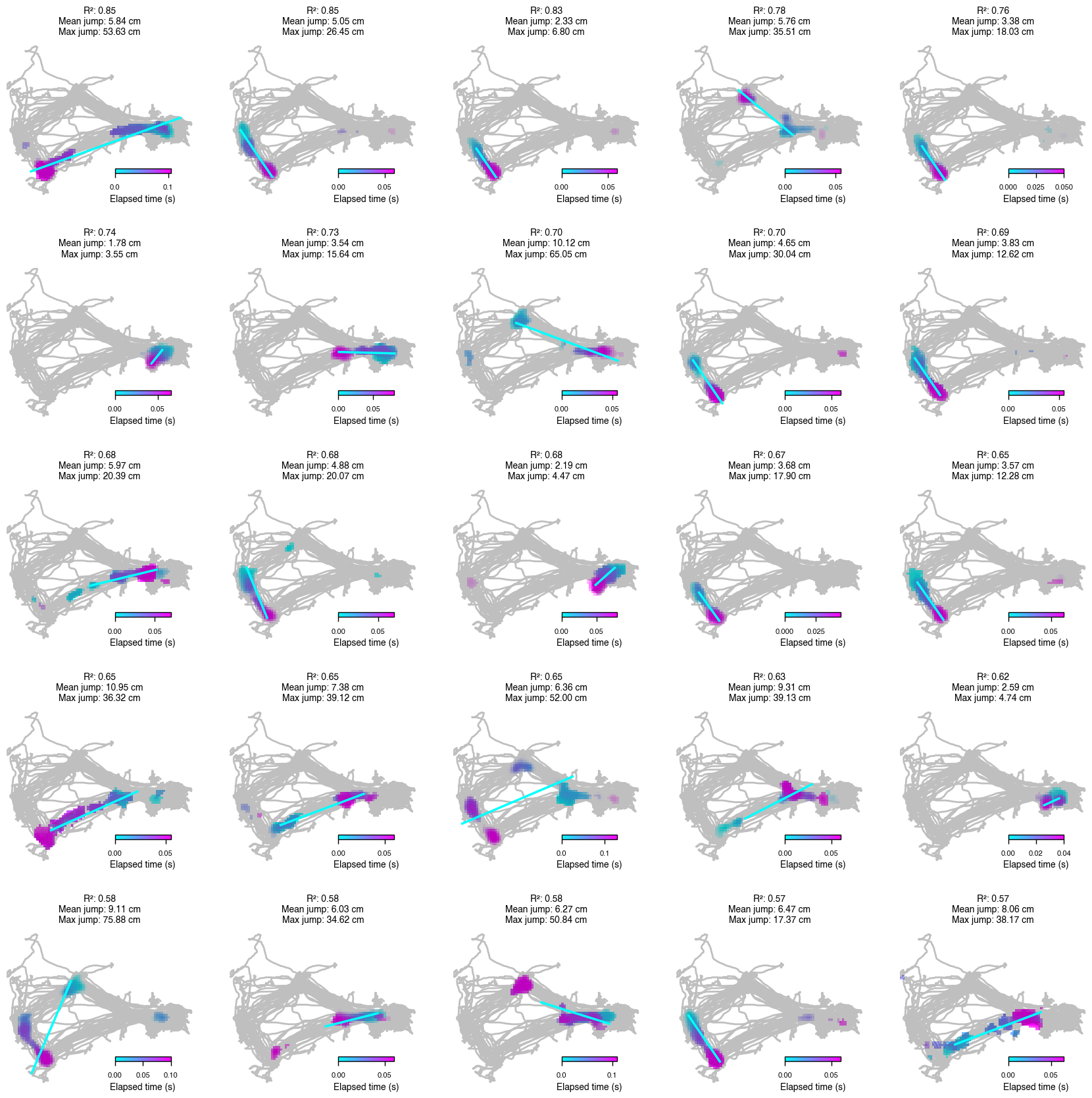
plot potential replays and fit lines¶

Titles report R² and jump distances in cm. The jump < 12 display filter uses mean jump distance in cm; it is not a replay significance test.

if RUN_REAL_DATA:
    from mpl_toolkits.axes_grid1.inset_locator import inset_axes

    npy.plotting.set_plotting_defaults()

    x, y = pos[beh_epochs[TASK_EPOCH]].data

    fig, ax = plt.subplots(
        5,
        5,
        figsize=npy.plotting.set_size("nature_double", fraction=1.5, ratio=1),
        dpi=200,
    )
    ax = ax.flatten()
    # Ripple IDs are labels, not positions in the compact score arrays.
    results_by_ripple = potential_replays.set_index(
        "ripple_index", verify_integrity=True
    )
    ripple_index_potential = (
        potential_replays.query("jump < 12")
        .sort_values("regression_r2", ascending=False)
        .ripple_index.values
    )

    for i, rid in enumerate(ripple_index_potential[:25]):
        event = results_by_ripple.loc[rid]
        posterior_ripple = posterior_prob[:, :, ripple_index == rid]
        ax[i].plot(x, y, color="k", alpha=0.25, zorder=2)

        npy.plotting.plot_2d_replay(
            posterior_ripple,
            extent=[
                spatial_maps.bins[0][0],
                spatial_maps.bins[0][-1],
                spatial_maps.bins[1][0],
                spatial_maps.bins[1][-1],
            ],
            saturation=5,
            ax=ax[i],
        )

        # plot fit line
        t = np.arange(posterior_ripple.shape[2], dtype=float) * SLIDE_BY
        t_centered = t - t.mean()
        x_fit = event["mean_x"] + event["slope_x"] * t_centered
        y_fit = event["mean_y"] + event["slope_y"] * t_centered
        ax[i].plot(x_fit, y_fit, color="cyan", lw=1.25, zorder=4)

        ax[i].set_title(
            f"R²: {event['regression_r2']:.2f}\n"
            f"Mean jump: {event['jump']:.2f} cm\n"
            f"Max jump: {event['max_jump']:.2f} cm",
            fontsize=5,
        )

        # Colorbar
        cmap = matplotlib.colormaps.get_cmap("cool").resampled(posterior_prob.shape[2])
        norm = colors.Normalize(vmin=0, vmax=posterior_ripple.shape[2] * SLIDE_BY)
        sm = mpl_cm.ScalarMappable(norm=norm, cmap=cmap)
        sm.set_array([])

        cax = inset_axes(
            ax[i], width="30%", height="3%", loc="lower right", borderpad=2
        )
        cbar = plt.colorbar(sm, cax=cax, orientation="horizontal")
        cax.xaxis.set_label_position("bottom")
        cax.set_xlabel("Elapsed time (s)", fontsize=5, labelpad=2)
        cbar.ax.tick_params(labelsize=4)

        ax[i].axis("off")
    for unused_ax in ax[min(25, len(ripple_index_potential)) :]:
        unused_ax.set_visible(False)
    plt.show()

png